Backpropagation

• Back-propagation is another name given to finding the gradient descent of the cost function in a neural network

  • That is we use the output error weights to refine the ANN weightings (next)
  • The gradient allows us to minimise the error rate

• Back-propagation can be used on supervised or unsupervised networks

• Our aim is to learn from the outputs

  • We iterate by tweaking values, learning which weightings decrease the error rate, which increase

1. The initial output is compared to the expected outputs and the weights adjusted to minimise this difference
2. Calculus (derivatives) is used to find the error gradient in the obtained output to adjust each neuron’s weights
3. Once we have reached no errors (or acceptable limits) we can determine that the network model is functioning
4. If the errors are still too large, the process is repeated until satisfactory

Types of Back-propagation (probably not in the exam) §

• Static back-propagation
  • The static back-propagation maps a static input for static output and is mainly used to solve static classification problems such as optical character recognition (OCR). The inputs and outputs are fixed and known
  • Moreover, here mapping is more rapid and compared to recurrent
• Recurrent back-propagation
  • This is the second type of back-propagation, where the mapping is non-static. It is fed forward until it achieves a fixed value, after which the error is computed and propagated backward
    • This is needed in dynamic systems where the data is continually changing

Minima §

• Gradient descent is an efficient optimisation algorithm that attempts to find a local or global minimum of the cost function
  • The cost function being something we want to minimise

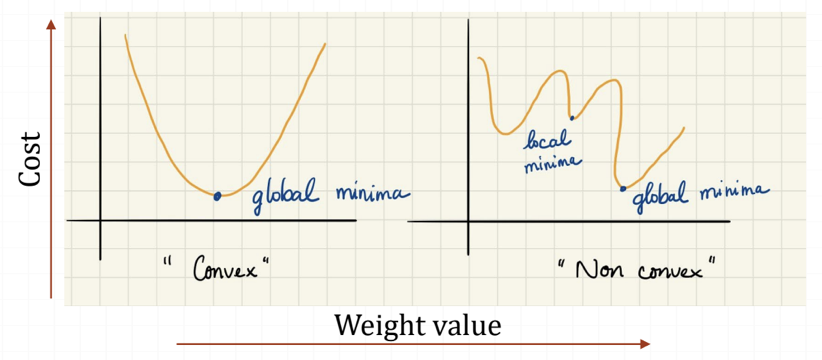
• A local minimum is a point where out function is lower than all neighbouring points
• A global minimum is a point that obtains the absolute lowest value of our function, but global minima are difficult to compute in practice